Weighted averaged, also known as weighted arithmetic mean, is similar to an ordinary average, except that instead of each of the data points contributing equally to the final average, each data point is “weighted” and thus contributes more or less depending on the given weight.  The weight would typically be some correlated data point that indicates significance of the value being averaged.

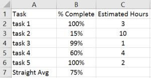
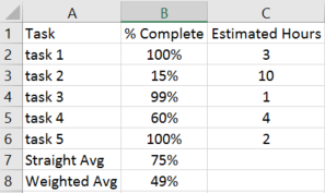
For example, let’s say we were tracking the progress of a project and its various tasks.  Our data set includes the task number, percent completed, and estimated hours to complete the task.  We want to calculate an overall percent completed for the project based on how complete the individual tasks are.  Take a look at the example below.

=AVERAGE(B2:B6)

If we calculate a straight average of the percent complete column then we get 75% completed overall.  However, this could be deceiving because some tasks will take longer to complete than others, as indicated in the estimated hours column.  Let’s use this estimated hours column as the “weight” in our weighted average.

One way to do this would be to:

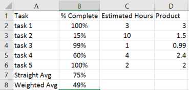
• multiply the item (% Complete) by the weight (Estimated Hours) at the row level, shown in column D below.
• sum up all of those products in column D, and then
• divide by the sum of the weight for all records (column C)

Formulas:

Results:

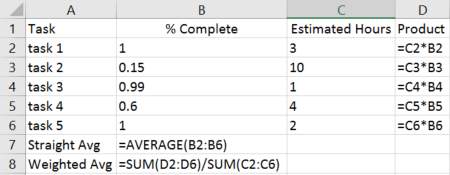
The result of the weighted average is 49%, which is much different than the 75% from a straight average.  This is because there are items which have a high percent completed but a low estimated hours to complete, and also items with low percent completed and higher estimated hours to complete.  By including a weight to factor in the level of effort for each item you get a much more accurate result.

What’s the problem with this approach? If the number of tasks changes then it becomes a fairly manual task to adjust the rows and formulas accordingly.  Also, I don’t like the idea of having a “helper” or “work” column inserted into the data set.  There is a quicker and simpler way to calculate the weighted average than the method I just explained.

In excel 2007 and forward there is a function called SUMPRODUCT(), which allows us to skip the step of calculating the weighted product for each row at the row level.  As its name suggests, this function multiplies corresponding components in given arrays, and returns the sum of those products.  In my example I supply two arrays of data, but the function will accept more in case you wanted to use more than one column as a weight.

Formulas:

Results:

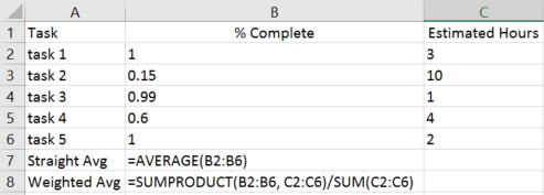
As you can see, this simplifies the calculation into a single cell and avoids odd features like array formulas, which I purposely omitted in this post.

For more information and examples on the sumproduct() function please visit the microsoft link here.